In this tutorial we would be looking at the dataset provided by IIT Madras for their 'Cricket Hackathon', and using some basic analysis tools to clean and engineer the data as we require. The contest is open for registrations, and you can do the same or read more at the link below.

IIT Madras Cricket and Coding Contest

Download the given dataset from the Contest Details tab, unzip it, and open any given file using Google Sheets or MS Excel, and you will find ball-by-ball data of all the games played in the IPL from 2008-2020. There are match files for each game, but we would be working with the all_matches.csv file that contains all the games together.

This single file has more than 1,94,000 lines of data, which may seem a lot to someone who is new, but is really really low by machine learning standards. So don't worry, you would encounter larger datasets in your data science career.

Open Google Colaboratory from your favourite browser, which allows anybody to write and execute arbitrary python code through the browser, and is very well suited to machine learning, data analysis and education. Sign in using your Google Account, click on New Notebook and once the instance is connected, you are good to go.

Google Colab

To begin with, save the dataset on your Google Drive, and mount Drive in Google Colab from the left pane. Now we write the first line of code by importing Pandas, which is a fast data analysis library for Python and has almost everything we would need to begin with. Add the path to your file in the pd.read_csv() function. Here is an example. This line saves the dataset in a dataframe named match_data.

import pandas as pd

match_data = pd.read_csv('drive/MyDrive/dataset/all_matches.csv')

To see what our new dataframe contains, we can take a glimpse of the data using the df.head() function.

match_data.head()

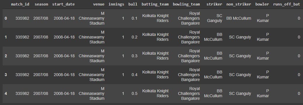
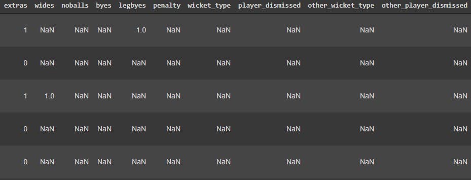
The output shows the first five rows of the dataset that we have imported. Let us now check all the columns, and check how many attributes of this dataset are numerical and categorical. We do this using the df.info() function.

match_data.info()

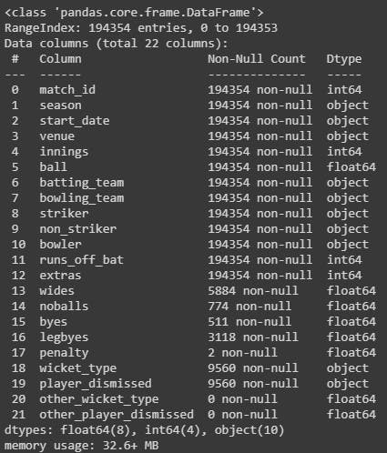
From the above two commands, and their respective outputs, we can make the following inferences about the data.

1. There are a total of 194353 deliveries that have been bowled in the dataset given to us.
2. match_id is a unique integer value for every match that has been played in the tournament throughout.
3. season, start_date and venue describe when and where the match was played.
4. innings is an integer value that depicts which half of the match is being played when a delivery is being recorded. We expect this variable to take only two values, 1 and 2, but we would look more into it later.
5. ball is a decimal value, that tells us which ball of the innings is being bowled. It starts from 0.1 which means the first over is the 0th integer, and the first ball is the 1st decimal part. Ideally, an over should have 6 balls but it may increase based on the number of extras and penalties the bowling team concedes.
6. batting_team, bowling_team, striker, non_striker and bowler are string categorical variables, and are very self-explanatory.
7. runs_off_bat and extras tells us the number of runs scored on that delivery, and the mode of that run.
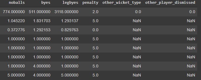
8. wides, noballs, byes, legbyes and penalty demonstrate the way the extra runs came from.
9. wicket_type and other_wicket_type tells us how a wicket fell, if it did, on a particular ball. This shows that there could be two wickets falling on the same delivery, which is a rare case scenario and happens when a wicket falls and a person retires on the same delivery, but we would have to keep this in mind.
10. player_dismissed and other_player_dismissed would again be a categoricla string variable that tells us the name of the batsmen dismissed on a particular delivery.

We do notice that there are not a lot of numerical attributes, but anyway, let us try to gain some more statistical insights using df.describe and see if we can learn something new.

match_data.describe()

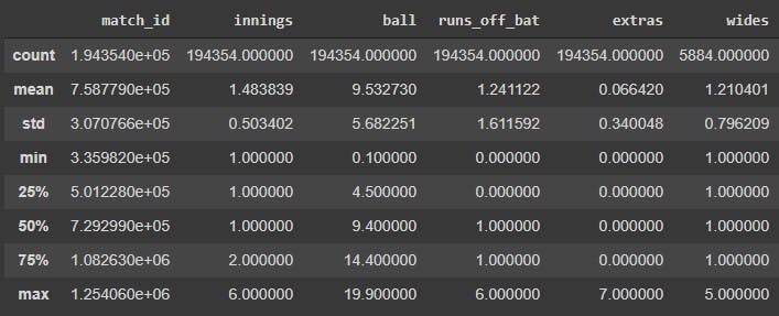
Time for some more inferences lads, here we go.

1. Since most numerical attributes are also categorical in nature, like innings or match_id, not a lot of the numbers here make sense.
2. But if you look carefully, the maximum innings played in a game is 6, which is not standard. This is because the matches that end in a tie go to a super over, which is a one over match. There can be a maximum of two super overs in a match, and thus, the total number of innings goes upto 6. We would have to take care of this later.
3. No player has been dismissed via retired hurt on the same ball as another wicket, so we can be sure that there is a maximum of only one dismissal on a delivery. However, we do need to take care of this case, however niche it may be, so that our data anaysis and machine learning has a universal approach to it.

This step, however boring it may seem, is called Data Exploration, and is an important step to learn the context of the numbers/variables we look at in the dataset, and identify any outliers that may hinder us later.

In the next part, we would discuss the combinations and operations on attributes inside a dataframe. We would also look at the test input data and the expected output format, and engineer this large dataset into a smaller and cleaner dataset, that is more useful and feature rich.