Welcome back! In the last part we looked at how to load the data in a Python environment, and how to do a basic exploration. Do make sure you read that before you start reading this one. I'll be waiting. :)

Moving on, let us try applying some basic data transformation techniques to gain more information and to quantify some attributes.

One of the most important aspects of data science and data analysis, is understanding the context in which the data is present. This is why we need a fairly deep knowledge of cricket as a sport before we can make sense of tons of random numbers and words.

Let us begin by looking at the input format provided by the contest page, to see what data would go into our model, and what needs to come out. Download the input_test_data.csv file from the contest page, upload it on your drive and access it using the same technique we used in the last blog. We also need to specify the delimiter='\t' argument here, as mentioned on the contest page. Read the official documentation of Pandas to find what this argument does.

sample_input_data = pd.read_csv('drive/MyDrive/dataset/sample_input_data.csv', delimiter='\t')
sample_input_data.head()

Thus, we find out that the sample input file that goes into our 'model' would have the venue, the innings, the ball, the teams playing and the players who have batted and bowled in the first six overs.

The problem statement asks us to predict the scores at the end of the sixth over, given the abovementioned inputs. Thus, we don't need the deliveries after the sixth over in our huge dataset. So let us trim that down to contain the deliveries only upto the sixth over of each innings.

match_data = match_data[match_data['ball'] < 6.0]

We know that the ball number 6.1 would be the first ball of the seventh over, so we trim the dataset to only contain the balls before that.

Let us add another column, for the total runs scored on a ball. We can do this by adding the runs scored off the bat and the extras for each delivery.

match_data['total_runs'] = match_data['runs_off_bat'] + match_data['extras']

Now let's make the initial dataset that we had, smaller. We don't need all the various columns that we had, so let us trim our dataset to include only the columns that interest us. Also, we don't really need a data that is divided delivery wise, so let us add all the runs scored in an innings, and store that row-wise.

match_data = match_data.groupby(['match_id', 'venue', 'innings', 'batting_team', 'bowling_team']).agg(total_runs = ('total_runs','sum'), wickets = ('wicket_type', 'count'),).reset_index()

This is a complex transformation an so could seem like a lengthy piece of code, but it is really simple. We are using df.groupby() to group datapoints by the identifiers given, then using df.groupby().agg() to sum the number of runs scored, and count the number of wickets.

Notably enough, I have not kept the list of batsmen and the list of bowlers in this new dataset because they did not seem a factor that can be quantified into the impact it has on a team's score. There are definitely some bowlers and batsmen who can have a serious impact on a team's score, but stochastic and condition-based approaches are not very appreciated in the data science community in general. That being said, feel free to play with the data whichever way you love to.

Also, because we have not yet taken care of the innings that are played in a super over, let us trim that part of the data as well, so that only the first two innings of a match remains a part of this cleaned dataset.

match_data = match_data[match_data['innings'] < 3]

Let us finally take a look at the new data that we have.

match_data.head()

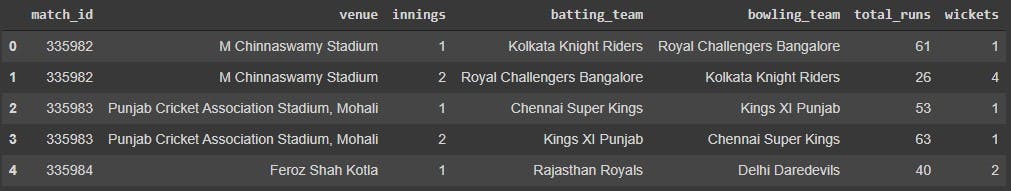
This now looks like a reasonable enough dataset to us. In fact, cricket freaks would remember that RCB indeed lose 4 wickets on 26 runs in the inaugural match of IPL 2008, so we can be fairly confident that this is an accurate dataset.

Pro Tip : Save your dataframe to your drive using to_csv() when you want to pause your work. This way you would not need to re-run all the commands, and you can have a restore point in case the server or your computer loses connection.

match_data.to_csv(r'drive/MyDrive/dataset/new_dataset.csv', index=False)

Run df.info() on this new dataset to see some details.

match_data.info()

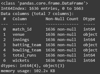
We can see that we are now left with the data of 1636 innings, and there seem to be no missing values. This is an important check to ensure the model doesn't run into any errors later on.

Run df.describe() to gain insights on the numerical attributes.

match_data.describe()

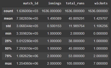
Here are the takeaways from the output.

1. The average number of runs scored by a team in the first six overs is 45.81, which could be a good first guess for a team's powerplay score.

2. The maximum number of runs scored in the first 6 overs is 105, and the maximum number of wickets conceded is 7.

Do comment below if you know which teams hold these records, against which opponents and in which season.

Also, let us look at some properties of the categorical variables as well. Since we know all the batting teams would also have bowled, let us look at the total number of batting teams, and the number of times they have appeared.

match_data['batting_team'].value_counts()

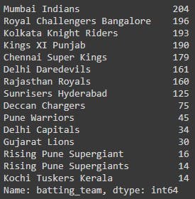
We see that there is a team that is repeated due to wrong data collection methods, and we can tackle this using the df[].replace() method. Since a wrong data entry would reflect both in the batting and the bowling team, let us replace both of these.

match_data'batting_team'] = match_data['batting_team'].replace('Rising Pune Supergiant', 'Rising Pune Supergiants')
match_data['bowling_team'] = match_data['bowling_team'].replace('Rising Pune Supergiant', 'Rising Pune Supergiants')

Do a value_counts() on the venue attribute, and see what different venues have games been played upon. Check if there are any duplicate names, and correct it using the method given above.

We did some rigorous data cleaning in this blog, and the data seems good enough for usage now. In the following blog, we would plot some colourful 2D graphs to visualise the data using Matplotlib. This way, we would analyse team wise scores and see if we can notice any visual patterns.